信息论2-交叉熵和散度

同步于CSDN;音尘杂记

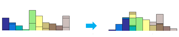
主要总结了交叉熵、KL散度、JS散度和wasserstein距离(也称推土机距离，EMD)的相关知识，其中EMD的直观表示可以参见下图：

1. 交叉熵

对应分布为$p(x)$的随机变量，熵$H(p)$表示其最优编码长度。交叉熵（Cross Entropy）是按照概率分布$q$的最优编码对真实分布为$p$的信息进行编码的长度，

交叉熵定义为

$$H(p, q) = \Bbb{E}_p[−log q(x)] = −\sum_{x}p(x)logq(x) \tag{1}$$

在给定$p$的情况下，如果$q$和$p$越接近，交叉熵越小；如果$q$和$p$越远，交叉熵就越大。

2. KL散度

KL散度（Kullback-Leibler Divergence），也叫KL距离或相对熵(Relative Entropy)，是用概率分布q来近似p时所造成的信息损失量。KL散度是按照概率分布q的最优编码对真实分布为p的信息进行编码，其平均编码长度$H(p, q)$和$p$的最优平均编码长度$H(p)$之间的差异。对于离散概率分布$p$和$q$，从$q$到$p$的KL散度定义为

$$D_{KL}(p∥q) = H(p,q) − H(p) = \sum_{x}p(x)log\frac{p(x)}{q(x)} \tag{2}$$

其中为了保证连续性，定义$0 log \frac{0}{0} = 0, 0 log \frac{0}{q} = 0$。

KL散度可以是衡量两个概率分布之间的距离。KL散度总是非负的，$D_{KL}(p∥q) ≥0$。只有当$p = q$时，$D_{KL}(p∥q) = 0$。如果两个分布越接近，KL散度越小；如果两个分布越远，KL散度就越大。但KL散度并不是一个真正的度量或距离，一是KL散度不满足距离的对称性，二是KL散度不满足距离的三角不等式性质。

3. JS散度

JS散度（Jensen–Shannon Divergence）是一种对称的衡量两个分布相似度的度量方式，定义为

$$D_{JS}(p∥q) = \frac{1}{2}D_{KL}(p∥m) + \frac{1}{2}D_{KL}(q∥m) \tag{3}$$

其中$m = \frac{1}{2}(p + q)$。

JS 散度是KL散度一种改进。但两种散度都存在一个问题，即如果两个分布p, q 没有重叠或者重叠非常少时，KL散度和JS 散度都很难衡量两个分布的距离。

4. Wasserstein距离

Wasserstein 距离（Wasserstein Distance）也用于衡量两个分布之间的距离。对于两个分布$q_1, q_2，p^{th}-Wasserstein$距离定义为

$$W_p(q_1, q_2) = \left ( \inf_{\gamma(x, y) \in \Gamma(q_1, q_2)}\Bbb{E}_{(x,y)\sim \gamma(x,y)}[d(x,y)^p] \right )^{1/p} \tag{4}$$

其中$Gamma(q_1, q_2)$是边际分布为$q_1$和$q_2$的所有可能的联合分布集合，$d(x, y)$为$x$和$y$的距离，比如$\ell_p$距离等。

如果将两个分布看作是两个土堆，联合分布$\gamma(x, y)$看作是从土堆$q_1$的位置$x$到土堆$q_2$的位置$y$的搬运土的数量，并有

$$\begin{eqnarray} \sum_{x}\gamma(x, y) = q_2(y) \tag{5} \\ \sum_{y}\gamma(x, y) = q_1(x) \tag{6} \end{eqnarray}$$

$q_1$和$q_2$为$\gamma(x, y)$的两个边际分布。

$\Bbb{E}_{(x,y) \sim \gamma(x,y)}[d(x, y)^p]$可以理解为在联合分布$\gamma(x, y)$下把形状为$q_1$的土堆搬运到形状为$q_2$的土堆所需的工作量，

$$\Bbb{E}_{(x,y) \sim \gamma(x,y)}[d(x, y)^p] = \sum_{(x,y)}\gamma(x, y)d(x, y)^p \tag{7}$$

其中从土堆$q_1$中的点$x$到土堆$q_2$中的点$y$的移动土的数量和距离分别为$\gamma(x, y)$和$d(x, y)^p$。因此，Wasserstein距离可以理解为搬运土堆的最小工作量，也称为推土机距离（Earth-Mover’s Distance，EMD）。

Wasserstein距离相比KL散度和JS 散度的优势在于：即使两个分布没有重叠或者重叠非常少，Wasserstein 距离仍然能反映两个分布的远近。

对于$\Bbb{R}^n$空间中的两个高斯分布$p = \cal{N}(\mu1,Σ1)$和$q = \cal{N}(\mu2,Σ2)$，它们的$2^{nd}-Wasserstein$距离为

$$D_W(p∥q) = ||μ1 − μ2||_2^2 + tr \left ( \begin {matrix} \sum_1 + \sum_2 - 2(\sum_2^{1/2}\sum_1\sum_2^{1/2})^{1/2} \end {matrix} \right ) \tag{8}$$

当两个分布的的方差为0时，$2^{nd}-Wasserstein$距离等价于欧氏距离($||μ1 − μ2||_2^2$)。

4.1 EMD示例

求解两个分布的EMD可以通过一个Linear Programming（LP）问题来解决，可以将这个问题表达为一个规范的问题：寻找一个向量$x \in \Bbb{R}$，最小化损失$z = c^Tx, c\in \Bbb{R}^n$，使得$Ax = b, A \in \Bbb{R}^{m\times n},b \in \Bbb{R}^m, x \geq 0$，显然，在求解EMD时有：

$$x = vec(\Gamma) \\ c = vec(D)$$

其中$\Gamma$是$q_1$和$q_2$的联合概率分布，$D$是移动距离。

首先生成两个分布$q_1$和$q_2$：

# -*- coding: utf-8 -*-
import numpy as np
import matplotlib.colors as colors
from matplotlib import pyplot as plt
from scipy.optimize import linprog
from matplotlib import cm
from scipy.optimize import linprog
from matplotlib import cm

l = 10

q1 = np.array([13, 8, 5, 1, 21, 15, 8, 7, 5, 15])
q2 = np.array([1, 6, 12, 17, 12, 10, 8, 15, 4, 2])
q1 = q1 / np.sum(q1)
q2 = q2 / np.sum(q2)

plt.bar(range(l), q1, 1, color='blue', alpha=1, edgecolor='black')
plt.axis('off')
plt.ylim(0, 0.5)
plt.show()

plt.bar(range(l), q1, 1, color='green', alpha=1, edgecolor='black')
plt.axis('off')
plt.ylim(0, 0.5)
plt.show()

计算其联合概率分布和距离矩阵：

D = np.ndarray(shape=(l, l))
for i in range(l):
    for j in range(l):
        D[i, j] = abs(range(l)[i] - range(l)[j])

A_1 = np.zeros((l, l, l))
A_2 = np.zeros((l, l, l))
for i in range(l):
    for j in range(l):
        A_1[i, i, j] = 1
        A_2[i, j, i] = 1

A = np.concatenate((A_1.reshape((l, l**2)), A_2.reshape((l, l**2))), axis=0)  # 20x100
b = np.concatenate((q1, q2), axis=0)  # 20x1
c = D.reshape((l**2))  # 100x1

opt_res = linprog(c, A_eq=A, b_eq=b, bounds=[0, None])
emd = opt_res.fun
gamma = opt_res.x.reshape((l, l))
print("EMD: ", emd)

# Gamma
plt.imshow(gamma, cmap=cm.gist_heat, interpolation='nearest')
plt.axis('off')
plt.show()

# D
plt.imshow(D, cmap=cm.gist_heat, interpolation='nearest')
plt.axis('off')
plt.show()

最终得到EMD=0.8252404410039889

4.2 利用对偶问题求解EMD

事实上，4.1节说的求解方式在很多情形下是不适用的，在示例中我们只用了10个状态去描述分布，但是在很多应用中，输入的状态数很容易的就到达了上万维，甚至近似求$\gamma$都是不可能的。

但实际上我们并不需要关注$\gamma$，我们仅需要知道具体的EMD数值，我们必须能够计算梯度$\nabla_{P_1}EMD(P_1, P_2)$，因为$P_1$和$P_2$仅仅是我们的约束条件，这是不可能以任何直接的方式实现的。

但是，这里有另外一个更加方便的方法去求解EMD；任何LP问题都有两种表示问题的方法：原始问题(4.1所述)和对偶问题。所以刚才的问题转化成对偶问题如下：

$$\begin {eqnarray} maxmize \qquad &\tilde{z}=b^T.y \\ st. \qquad &A^T.y \leq c \end {eqnarray} \tag{9}$$

opt_res = linprog(-b, A.T, c, bounds=(None, None))

emd = -opt_res.fun
f = opt_res.x[0:l]
g = opt_res.x[l:]

# print(dual_result)
print("dual EMD: ", emd)

得到其结果：EMD=0.8252404410039867

或者另一种方式：

emd = np.sum(np.multiply(q1, f)) + np.sum(np.multiply(q2, g))
print("emd: ", emd)

得到其结果，EMD=0.8252404410039877

最后，再看一下两个分布的对应转换情况：

# q1
r = range(l)
current_bottom = np.zeros(l)
cNorm = colors.Normalize(vmin=0, vmax=l)
colorMap = cm.ScalarMappable(norm=cNorm, cmap=cm.terrain)

for i in r:
    plt.bar(r, gamma[r, i], 1, color=colorMap.to_rgba(r), bottom=current_bottom, edgecolor='black')
    current_bottom = current_bottom + gamma[r, i]

plt.axis('off')
plt.ylim(0, 0.5)
plt.show()

# q2
r = range(l)
current_bottom = np.zeros(l)
for i in r:
    plt.bar(r, gamma[i, r], 1, color=colorMap.to_rgba(i), bottom=current_bottom, edgecolor='black')
    current_bottom = current_bottom + gamma[i, r]

plt.axis('off')
plt.ylim(0, 0.5)
plt.show()

主要参考:

• https://github.com/nndl/nndl.github.io
• https://vincentherrmann.github.io/blog/wasserstein/